ZGOUBI exercises
Describe quickly the content of the tutorial.
[updated: 2014-09-17]
Introduction to ZGOUBI: quick overview and main features
The computer code zgoubi calculates trajectories of charged particles in magnetic and electric fields.
Compared to other codes, it presents various peculiarities:
- a numerical method for integrating the Lorentz equation, based on Taylor series, which optimizes computing time and provides high accuracy and strong symplecticity,
- spin tracking, using the same numerical method as for the Lorentz equation,
- calculation of the synchrotron radiation electric field and spectra in arbitrary magnetic fields, from the ray-tracing outcomes,
- the possibility of using a mesh, which allows ray-tracing from simulated or measured (1-D, 2-D or 3-D) field maps,
- numerous Monte Carlo procedures: unlimited number of trajectories, in-flight decay, photon emission, etc.
- a built-in fitting procedure including arbitrary variables and a large variety of constraints,
- multiturn tracking in circular accelerators including features proper to machine parameter calculation and survey, simulation of time-varying power supplies,
Numerical Calculation Of Motion and Fields:
What Zgoubi does ?
Essentially, push a particle, step by step, in B or E fields.
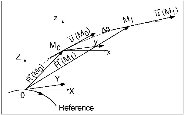
Position and velocity of a particle in the reference frame.
i.e., it numerically solves the Lorentz Equation:
How it does it ?
By using truncated Taylor expansions for position and normalized velocitiy
|
\vec R(M_1) & \approx \vec R(M_0) + \vec u(M_0)\, \Delta s+ \vec u^{\,\prime} (M_0)\,
\dfrac{\Delta s^2 }{2!} + ...+ \vec u^{\cinqprime} (M_0)\,
\dfrac{\Delta s^6 }{6!}
\vec u(M_1) & \approx \vec u(M_0) + \vec u^{\,\prime} (M_0)\,\Delta s + \vec u^{\,\prime\prime} (M_0)\,
\dfrac{\Delta s^2 }{2!} + ...+ \vec u^{\cinqprime} (M_0)\,
\dfrac{\Delta s^5 }{5!}
wherein |
require computation of the derivatives
so that the Lorentz equation can be re-written under the more convenient form (at least more convenient to handle in the code):
|
(B\rho )^\prime \vec u+\Br \,\vec u^{\,\prime}
= \frac{\vec e }{v} + \vec u \times \vec b
|
CYCLOTRON FIELDMAPS for ZGOUBI
Fieldmaps formatting: there are different types of field read functions that are already implemented in the code:1D/2D/3D, cartesian/cylindrical and many others.
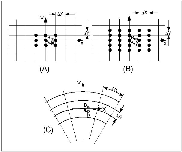
Mesh in the (X,Y) plane: the grid is centered on the node which is closest to the actual position of the particle.
The grid simply aims at interpolating the field and its derivatives at a given point from its 9 or 25 neighbors. For that, an interpolation polynomial (to the second or fourth order) is used.
In the special case of the optical element " POLARMES " (which will be used for this exercise), the field is given in Polar coordinates (case C above) in the median plane. Extrapolation off median plane is then performed by means of Taylor series (the median plane antisymmetry is assumed and the Maxwell equations accommodated).
The field map data file has to be filled with a format that fits the Fortran reading sequence.Details and possible updates are to be found in the source file " fmapw.f ". You should revise it to match your own field map format if it is different from the types already implemented.
Search for the closed orbits using the fitting routine in Zgoubi
CASE STUDY: PSI main ring cyclotron
• Change directory to ../FFAG14_workshop_tutorial/Search_CO/Zgoubi_CO
• Write down the following data list. Save it in "zgoubi.dat", it will be our input to zgoubi:
Search for the closed orbits using 'FIT2' keyword
 'OBJET'
1249.3978        !reference rigidity (kG.cm)
2                !option index (KOBJ)
1 1              !total number of particles  ;  number of distinct momenta
204.1173  8.9165  0.0   0.0  0.0  1.0  o   72MeV  !coordinates (Y(cm) T(mrad) Z(cm) P(mrad) X(cm) D(no dim)) and tagging
1 1 1 1 1 1

'PARTICUL'                                !particle characteristics
 938.2723   1.602176487D-19  0. 0. 0.     !mass, charge, gyromagnetic factor, COM life-time, unused

 'POLARMES'                                              	      !2D polar mesh magnetic field map
  0  0                                		   	    !print the map(1,2) ; print the field along trajectories(1,2,7)
  1. 1.00d0  1.                         		    	         !normalization coeff for B, A and R
  SECTOR  HEADER 4                    					 	    !TITLE
   136 140                                                     !number of angular and radial nodes of the mesh
 ../../Fieldmaps/Fieldmaps_Zgoubi/POLARMES_PSI_drift.H         !file name
  0  0. 0. 0.                                                  !integration boundary (ineffective)
   4                 					       !degree of interpolation polynomial
  1.                                                           !integration step
  2                                                            !KPOS
  0.  -0. 0. 0.                                                !RE,TE,RS,TS

'FIT2'                   !fitting procedure
2                        !number of physical parameters to be varied
1 30 0  [190,460]        !Vary initial coordinate Y0(horiz. position)
1 31 0  [-400,400]       !Vary initial coordinate T0(horiz. angle)
2   1.e-14  1000         !number of constraints, penalty, number of iterations
3.1 1 2 3 0. 1. 0        !define the 1st constraint (Y0=Y at exit of the magnet)
3.1 1 3 3 0. 1. 0        !define the 2nd constraint (T0=T at exit of the magnet)

'FAISTORE'   			!store coordinates every 1 pass in a file named rebeloteVersion.fai
orbitCoordinates.fai
1

'REBELOTE'               !multi re-do the FIT for 259 different rigidities
 259 0.1 0 1
 1                       !list of 259 successive values of D in OBJET follows
 OBJET  35     1.0143139       1.0284563       1.0424342       1.0562541       1.0699223       1.0834442       1.0968256       1.1100713       1.1231861       1.1361747       1.1490413       1.1617899       1.1744244       1.1869485       1.1993656       1.2116790       1.2238917       1.2360069       1.2480273       1.2599556       1.2717946       1.2835464       1.2952138       1.3067987       1.3183035       1.3297303       1.3410808       1.3523573       1.3635613       1.3746948       1.3857594       1.3967568       1.4076885       1.4185561       1.4293610       1.4401046       1.4507884       1.4614135       1.4719813       1.4824930       1.4929498       1.5033529       1.5137032       1.5240020       1.5342503       1.5444489       1.5545990       1.5647016       1.5747573       1.5847673       1.5947324       1.6046532       1.6145309       1.6243660       1.6341593       1.6439117       1.6536238       1.6632963       1.6729300       1.6825254       1.6920832       1.7016042       1.7110889       1.7205378       1.7299515       1.7393308       1.7486759       1.7579877       1.7672665       1.7765130       1.7857275       1.7949106       1.8040627       1.8131844       1.8222760       1.8313382       1.8403711       1.8493754       1.8583513       1.8672994       1.8762201       1.8851136       1.8939804       1.9028209       1.9116354       1.9204243       1.9291880       1.9379267       1.9466408       1.9553307       1.9639966       1.9726391       1.9812580       1.9898541       1.9984274       2.0069783       2.0155072       2.0240140       2.0324993       2.0409634       2.0494063       2.0578287       2.0662303       2.0746117       2.0829730       2.0913146       2.0996366       2.1079392       2.1162229       2.1244876       2.1327336       2.1409612       2.1491704       2.1573617       2.1655354       2.1736913       2.1818297       2.1899509       2.1980553       2.2061427       2.2142134       2.2222676       2.2303054       2.2383273       2.2463331       2.2543232       2.2622976       2.2702565       2.2782004       2.2861290       2.2940426       2.3019412       2.3098254       2.3176949       2.3255501       2.3333912       2.3412180       2.3490310       2.3568304       2.3646157       2.3723876       2.3801463       2.3878915       2.3956237       2.4033430       2.4110491       2.4187427       2.4264235       2.4340918       2.4417479       2.4493914       2.4570229       2.4646423       2.4722497       2.4798453       2.4874291       2.4950016       2.5025623       2.5101116       2.5176497       2.5251763       2.5326920       2.5401967       2.5476904       2.5551734       2.5626457       2.5701072       2.5775583       2.5849988       2.5924292       2.5998490       2.6072588       2.6146586       2.6220481       2.6294279       2.6367979       2.6441581       2.6515086       2.6588495       2.6661808       2.6735027       2.6808152       2.6881185       2.6954126       2.7026975       2.7099733       2.7172403       2.7244983       2.7317474       2.7389877       2.7462194       2.7534423       2.7606568       2.7678626       2.7750602       2.7822492       2.7894301       2.7966027       2.8037670       2.8109233       2.8180714       2.8252118       2.8323441       2.8394685       2.8465850       2.8536937       2.8607950       2.8678885       2.8749743       2.8820527       2.8891237       2.8961871       2.9032433       2.9102921       2.9173336       2.9243679       2.9313951       2.9384153       2.9454284       2.9524343       2.9594333       2.9664257       2.9734108       2.9803894       2.9873612       2.9943264       3.0012846       3.0082364       3.0151815       3.0221202       3.0290525       3.0359783       3.0428977       3.0498106       3.0567174       3.0636177       3.0705121       3.0774000       3.0842819       3.0911577       3.0980275       3.1048913       3.1117489       3.1186008       3.1254468       3.1322868       3.1391211       3.1459494       3.1527722       3.1595891       3.1664004       3.1732061       3.1800063       3.1868007       3.1935897       3.2003732       3.2071514       3.2139239       3.2206912

 'END'
• Run zgoubi which will output a file named "orbitCoordinates.fai" containing the initial coordinates of the closed orbits.
• Copy the trajectories in a new file named "CO.out" which will be used for the rest of the tutorial (in the right format used by Zgoubi). You can use the awk command for that:
awk '{print $10, $11, "0.0", "0.0", "0.0",$9+1.0, "'o'"}' orbitCoordinates.fai > CO.out
PS: A simple fortran routine that can be used to generate the different values of D (that were used in the input file) can be found in the Toolbox.
Plot the Closed Orbits (from zgoubi.plt file)
• Change directory to ../FFAG14_workshop_tutorial/Plot_Closed_Orbits
• Note the presence of a '2' (IL=2, following the users' guide nomenclture) right underneath 'POLARMES': This tells zgoubi to save particle data, step after step while stepwise ray-tracing, into zgoubi.plt.
• Using gnuplot you can plot the content of zgoubi.plt. Let's plot the field along some trajectories:
From a terminal, type
gnuplot < plot_field.gp &
• The results are shown below
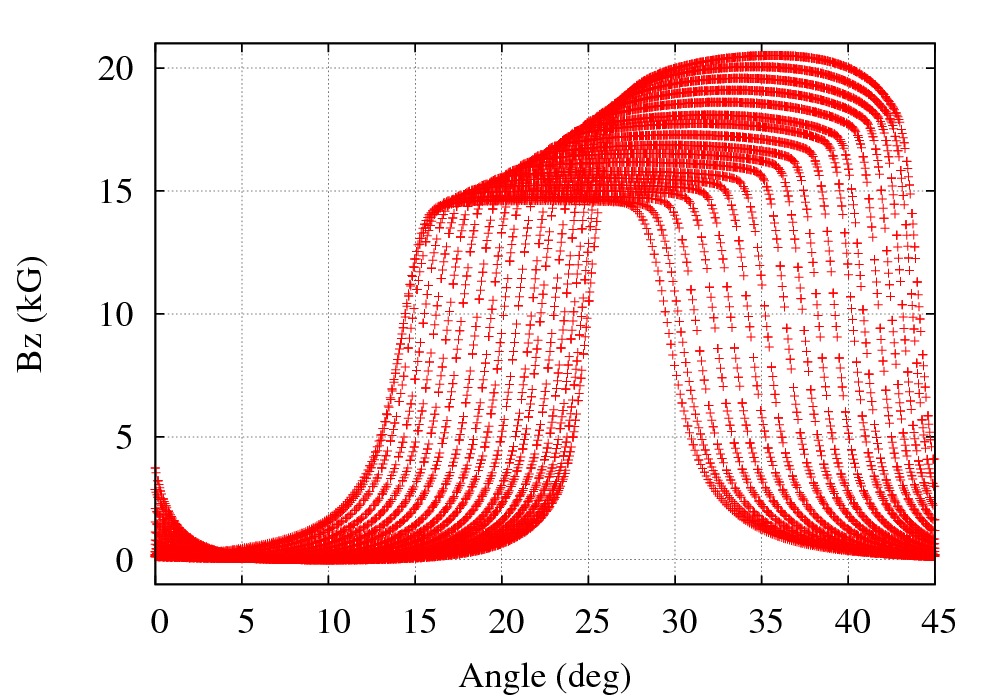
Bz(i.e. vertical) component of the magnetic field along trajectories step by step. across "POLARMES".
• We can also plot the closed orbits:
gnuplot < plot_orbits.gp &
which should output:
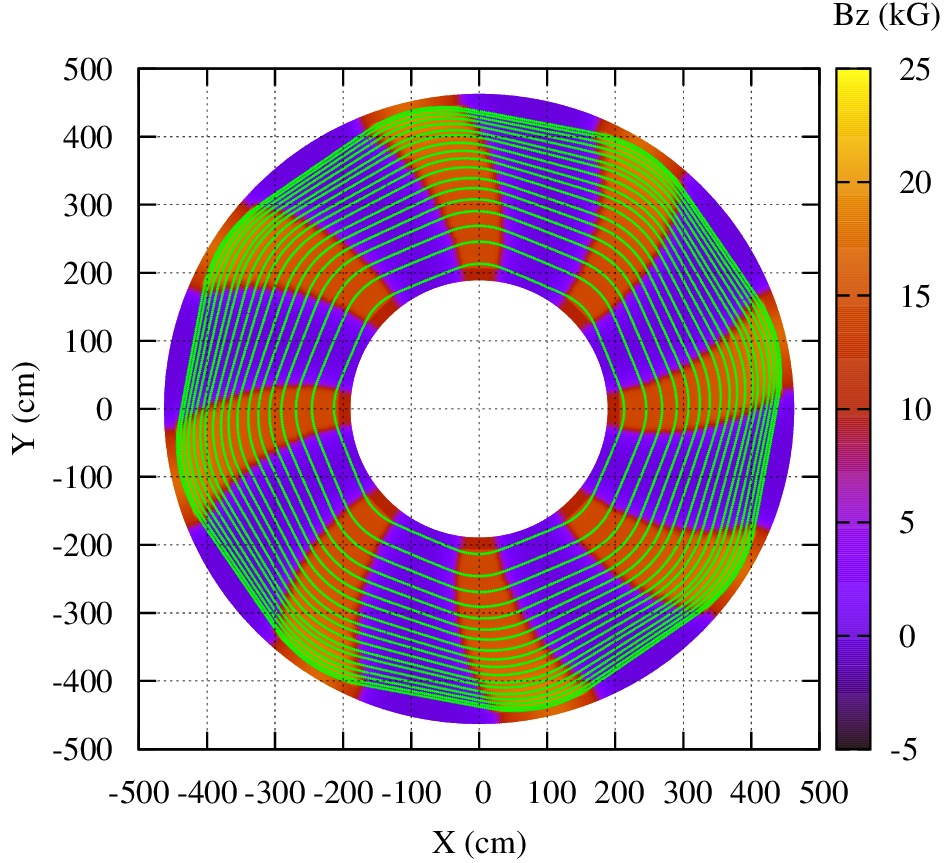
Plot of the closed orbits obtained from the measured median plane field map using "POLARMES".
• This is a fundamental thing to do, prior to going any further:
make sure the field experienced by the particles looks (reasonably) physical. Or, even better, exactly what you were expecting from the analytical calculations you did the night before.• This is a second fundamental thing to do, prior to going any further:
make sure the numerical integration does converge, i.e. :- integration step is small enough. Not too small yet because you do not want (i) to spend your life getting a particle transported, (ii) to reach computer truncature limit !!
- integration extends far enough in field fall-off regions that field has become negligible
Compute the Transfer Matrix for one sector
• Change directory to ../FFAG14_workshop_tutorial/Transfer_Matrix
• Run zgoubi.dat in order to obtain the transfer matrix of the sector: for that KOBJ=5.NN has to be chosen which will generate NN sets of 11 particles: for each set the initial coordinates (of the 11 particles) are taken wrt to the reference. A subsequent use of the keyword MATRIX would cause the computation of NN transport matrices.
• Search for the keyword "MATRIX" in zgoubi.res file. A typical output of MATRIX is displayed below,
************************************************************************************************************************************
      4  Keyword, label(s) :  MATRIX


  Reference, before change of frame (part #     1)  :
   0.00000000E+00   2.04117116E+02   8.91733417E+00   0.00000000E+00   0.00000000E+00   1.64852706E+02   1.48317496E-02

           Frame for MATRIX calculation moved by :
            XC =    0.000 cm , YC =  204.117 cm ,   A =  0.51093 deg  ( = 0.008917 rad )


  Reference, after change of frame (part #     1)  :
   0.00000000E+00   0.00000000E+00   0.00000000E+00   0.00000000E+00   0.00000000E+00   1.64852706E+02   1.48317496E-02

  Reference particle (#     1), path length :   164.85271     cm  relative momentum :   1.000000


                  TRANSFER  MATRIX  ORDRE  1  (MKSA units)

          0.605885         1.33020         0.00000         0.00000         0.00000        0.633577
         -0.465679        0.616639         0.00000         0.00000         0.00000        0.750330
           0.00000         0.00000        0.757019         1.47005         0.00000         0.00000
           0.00000         0.00000       -0.286059        0.765476         0.00000         0.00000
          0.740630        0.605014         0.00000         0.00000        1.000000        7.697620E-02
           0.00000         0.00000         0.00000         0.00000         0.00000        1.000000

          DetY-1 =      -0.0069408246,    DetZ-1 =       0.0000007690

          R12=0 at   -2.157     m,        R34=0 at   -1.920     m

      First order symplectic conditions (expected values = 0) :
        -6.9408E-03    7.6899E-07     0.000         0.000         0.000         0.000


                TWISS  parameters,  periodicity  of   1  is  assumed
                                    - UNCOUPLED -

       Beam  matrix  (beta/-alpha/-alpha/gamma) and  periodic  dispersion  (MKSA units)

           1.690151     0.006832     0.000000     0.000000     0.000000     1.596164
           0.006832     0.591691     0.000000     0.000000     0.000000     0.000866
           0.000000     0.000000     2.266979     0.006520     0.000000     0.000000
           0.000000     0.000000     0.006520     0.441134     0.000000     0.000000
           0.000000     0.000000     0.000000     0.000000     0.000000     0.000000
           0.000000     0.000000     0.000000     0.000000     0.000000     0.000000

                                   Betatron  tunes

                    NU_Y =  0.14490186         NU_Z =  0.11229365
• Another way to make sure that the tracking finished well is to check the symplectic conditions: the expected values must be close to 0 as obtained here:
      First order symplectic conditions (expected values = 0) :
        -6.9408E-03    7.6899E-07     0.000         0.000         0.000         0.000
• The beta matrix (that ensures the 8-fold symmetry of the ring) as well as the tunes are computed here as well.
Plot the Beam Envelope
• Change directory to ../FFAG14_workshop_tutorial/Beam_Envelope
• Copy the content of the file "zgoubi.dat_Vertical_Envelope" into "zgoubi.dat"
• Edit "zgoubi.dat": Use KOBJ=8 (in the element "OBJET") in order to generate phase space coordinates: the ellipse parameters at the start of the tracking are obtained from "MATRIX" calculation (previously detailed) which ensures a periodic solution to the problem (no acceleration).
• Use gnuplot to plot the axial beam envelope:
gnuplot < plot_axi_env.gp &
which should output:
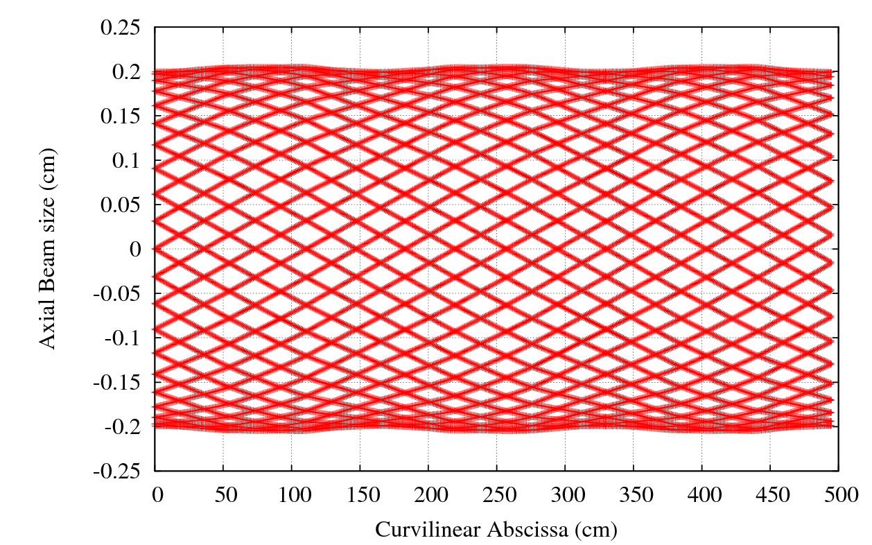
Axial beam envelope at injection (72 MeV) for 3 sectors.
• Compile and run the file "plot_radial_envelope.f". It will output a file named "envelope" which contains the data needed to plot the radial beam envelope.
• Use gnuplot to plot the radial beam envelope:
gnuplot < plot_rad_env.gp &
which should output:
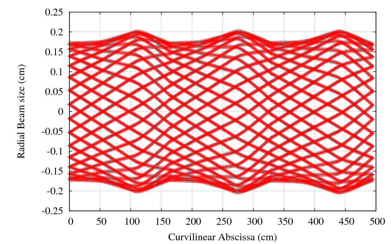
Radial beam envelope at injection (72 MeV) for 3 sectors.
Compute the Tunes
• Change directory to ../FFAG14_workshop_tutorial/Search_tunes
1) use the "CO.out" file and add a small increment in the radius and the angle to introduce small betatron oscillations around the closed orbit. You can use the awk command for instance from a terminal:
awk '{print $1+0.2, $2+0.3, $3+0.1, $4+0.3, $5, $6, $7}' CO.out > Orbit_tune.inp
2) track these particles in zgoubi which will output a file named "b_zgoubi.fai"
3) compile "tunesFromFai.f" in the sub-directory tunesFromFai. Then run "tunesFromFai" (from the directory Search_tunes) which uses the b_zgoubi.fai file and will output "tunesFromFai.out" containing many results among which the axial and radial tunes (ZZNU and XXNU respectively)
4) plot the tune results using gnuplot: from a terminal type
gnuplot < plot_tunes.gp &
The results are shown below:
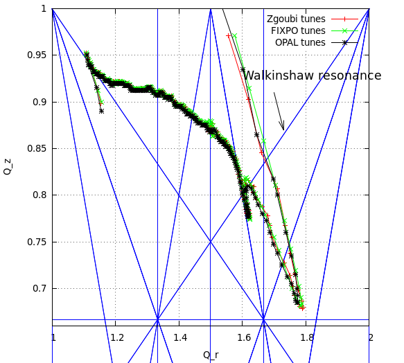
Tune diagram with the 3rd order resonance lines.
Cyclotron Model
CYCLOTRON semi-analytical model description• Change directory to ../FFAG14_workshop_tutorial/Cyclotron_model
• Copy the content of the file "zgoubi.dat_Vertical_Envelope" into "zgoubi.dat"
• Run "zgoubi.dat" which will generate a "zgoubi.plt" file that will be used to plot the field along some trajectories (that you choose).
• Plot the orbit trajectory obtained from "CYCLOTRON" with the definition of the Spiral boundaries:
gnuplot < plot_orbit.gp
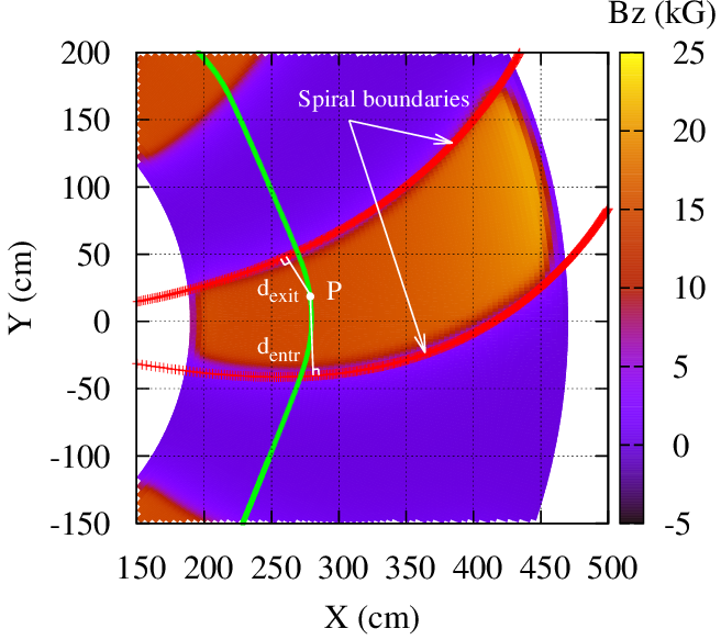
Orbit trajectory as obtained from "CYCLOTRON" model with some geometrical parameters used for the tracking.
• Plot the field along some trajectories:
gnuplot < plot_field.gp &
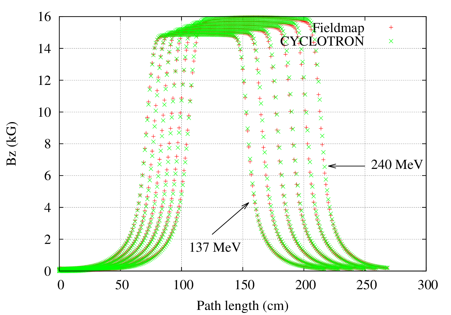
Comparison of the magnetic field along different trajectories (137, 156, 176, 196, 218 and 240 MeV) obtained from the tracking using the analytical model "CYCLOTRON" (in green) and from the fieldmap using "POLARMES" (in red) .
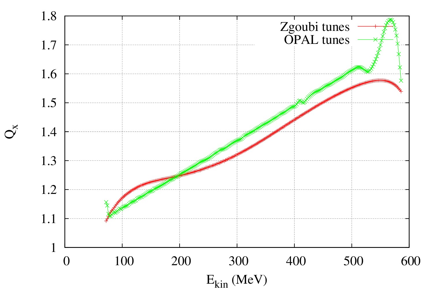
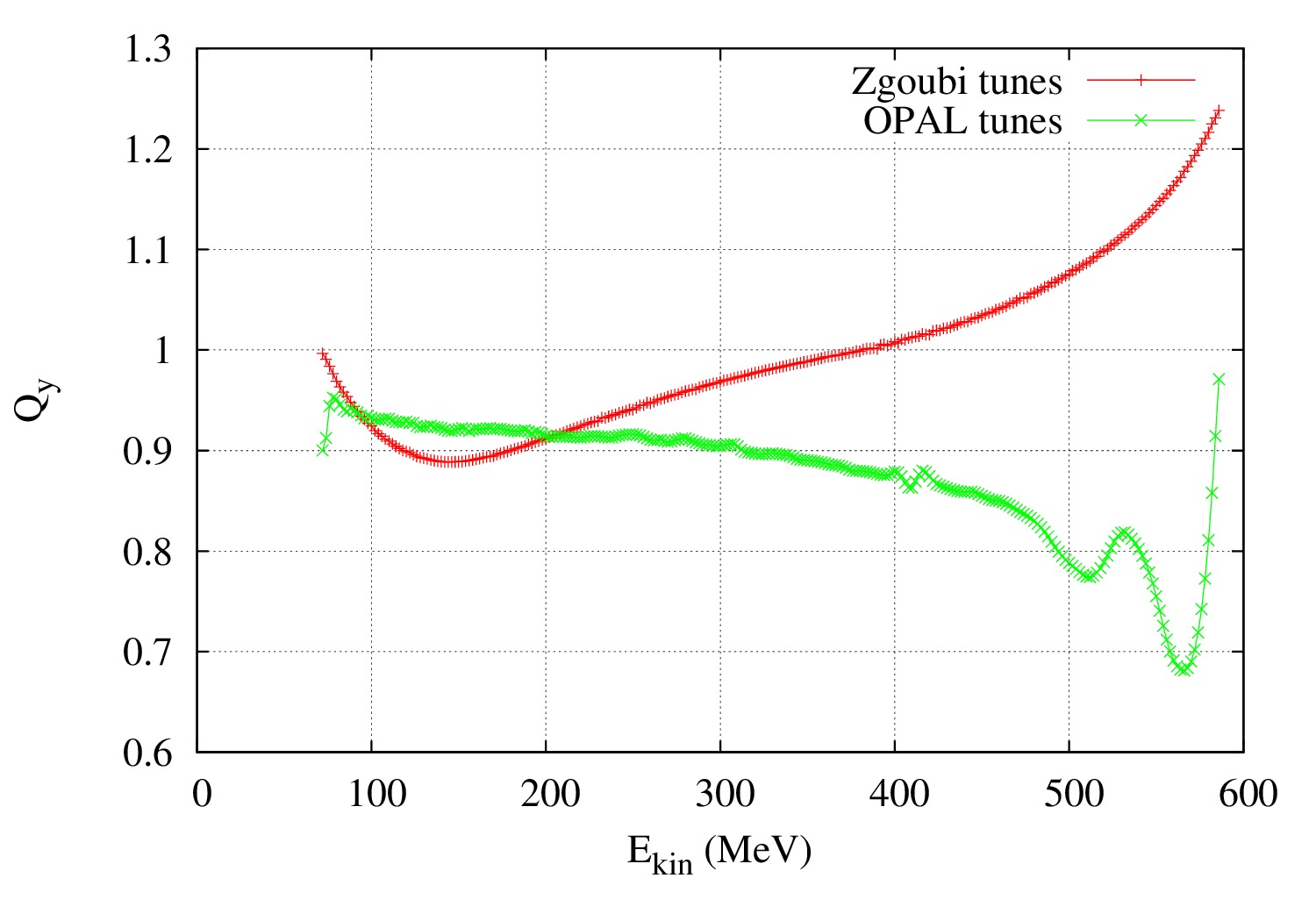
Radial (left) and axial (right) tune results as a function of the kinetic energy: the red lines show the tunes obtained from the "CYCLOTRON" model while the green one show the one obtained from the fieldmap. At higher energies the differences are important: this was expected as the fringe field coefficients used in the model were obtained for the orbit 137 MeV (see "CYCLOTRON semi-analytical model description" above). The fringe field coefficients should thus be allowed to change as a function of the radius.